Compound Annual Growth rate in Business Objects

To calculate the Compound Annual Growth rate, Excel has a function called XIRR. BO doesn't have that, but that's easy to remedy. All you need to do, is work out the following formula:

So, now we need a bunch of numbers and see where we get:

Right -- this has everything to do with investments, something I know nothing about, but here's some numbers to get us started :

On Jan 1 2010, we invest 10000€
On Jan 1 2011, our investment has grown to 13000€
On Jan 1 2012, our investment has grown to 15000€
and
finally, On Jan 1 2013, our investment has now a value of 19500€

The table looks like this in BO:

First, we'll divide our ending value by our beginning value -- interesting challenge.

Our last date would be : =Max([Date]) In Report = 1/1/2013

Our first date would be : =Min([Date]) In Report = 1/1/2010

So, our formula for that division becomes :

=[Value] where ([Date]=Max([Date]) In Report) / [Value] where ([Date]=Min([Date]) In Report)

I'll call this one basefigure

Now, we need to find out how many years it took:

The formula for that one is rather easy :

=Year(Max([Date]) In Report) - Year(Min([Date]) In Report)

And we divide 1 by that figure:

=1/(Year(Max([Date]) In Report) - Year(Min([Date]) In Report))

this one, I'll call exponent

There. Now, the next step would be to raise our first figure to the power of that second figure and subtract 1.

=Power([Basefigure];[Exponent])-1

Our Compound Annual Growth rate would be : 0.25 -- I guess those figures occurred in a parallel universe :)

Cool

Cheers folks

Peter

A running balance in Business Objects

I think it's quite clear by now, that it is my objective, never ever to need Excel -- well, almost. The charts in Excel do exceed BO's, but math -- naaaah.

Our next venture, is calculating a running balance.

In a running balance, we have a series of deposits and a series of withdrawals and we want to
keep track of the total of our balance at all times.

Here's how:

First, we need two columns. One has our deposits, the other has the withdrawals.

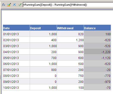
Now, we want to show a third column, with our balance -- on 1/1/2013, this should be : 180, on 2/1/2013, this should be -620 etc.

This is laughably easy really -- since BusinessObjects has a function Excel doesn't have: RunningSum

=runningsum([Deposit]) - runningsum([Withdrawal])

The result is :

In Excel this would be something like :

A	B	C
Deposits	Withdrawals	Balance
$1,000	$625	=SUM(A2,-B2)
$1000	740	=SUM(C2,A3,-B3)

Looks like our balance is in the red -- but with the economic times, that seems right :)

Cheers folks

Peter

The two most recent items (Business Objects)

This is going to be an easy one. Just a tip.

Let's assume, you want to know information for the two most recent pieces of data. Issue is, how do you get those most recent ones.

First, you need a measure -- based on a date.

Year([your_date]) this will get you the year, which is more than unique enough.
+Monthnumberinyear([your_date])/12

to the year, we add 1/12 of our month.

+daynumberinmonth([your_date])/31

and to that, we add 1/31 of the day.

The thing is, we don't want

15/March/2012

to be bigger than

1/April/2012

if we divide, we end up with numbers that stay in proportion.

An alternative, and probably an even better way to do this, is to multiply:

(Year([your_date])*10000) +    'that gives us 20120000
(Monthnumberinyear([your_date]) * 100)+   ' that gives us 201212
daynumberinmonth([your_date])  ' that should make 20121224

Interesting, it keeps the date readable. Which is always useful.



So, now we have our measure to base our ranking on -- now it's easy to get the two most recent ones isn't it.

Cheers.

Peter

Complex Query's

A participant of one of my courses provided me with the following intriguing question. For 1 given year, you need to know which stores both sold product A and B.
When you create the query where you choose both stores and the product and create a crosstab, you will also get results where one store sold something, and the other did not.


This picture shows what happens. There are occurences where one store sold something, and the other did not. Business Objects then shows “discontinued”.






The solution I found, is situated at the query level, and includes a combination of subquery’s and union query’s.
First, I created a query where I specify my first source :


it includes the name of the stores, the number of the product and the sales revenue. All of this is done using the eFashion universe, interesting for demonstration purposes only. The real work goes on in the conditions.
Storename and year are filtered as usual.
SKU number is filtered using a subquery. in this case, listing only the SKU numbers that are the result of that subquery.



The subquery looks like this :


The result of this query is a list of all SKUs sold in the other store. So we only get products in store A that have been sold in store B.
It is now possible to select both stores, but if we do that, then we will get some products for store B that were not sold in store A.. so not a good idea.
Next, we need to create a Union query, to also show data about the second store.



Click the  icon. It will add a second query, and you repeat the previous steps, but now for the other store. This means : the first query is then for Boston, the subquery for austin. The result looks like this :