Posts tonen met het label Calculation. Alle posts tonen

zondag, januari 27, 2013

Compound Annual Growth rate in Business Objects

To calculate the Compound Annual Growth rate, Excel has a function called XIRR. BO doesn't have that, but that's easy to remedy. All you need to do, is work out the following formula:

So, now we need a bunch of numbers and see where we get:

Right -- this has everything to do with investments, something I know nothing about, but here's some numbers to get us started :

On Jan 1 2010, we invest 10000€
On Jan 1 2011, our investment has grown to 13000€
On Jan 1 2012, our investment has grown to 15000€
and
finally, On Jan 1 2013, our investment has now a value of 19500€

The table looks like this in BO:


First, we'll divide our ending value by our beginning value -- interesting challenge.

Our last date would be : =Max([Date]) In Report = 1/1/2013
Our first date would be : =Min([Date]) In Report = 1/1/2010


So, our formula for that division becomes :

=[Value] where ([Date]=Max([Date]) In Report) / [Value] where ([Date]=Min([Date]) In Report)

I'll call this one basefigure


Now, we need to find out how many years it took:

The formula for that one is rather easy :

=Year(Max([Date]) In Report) - Year(Min([Date]) In Report)

And we divide 1 by that figure:

=1/(Year(Max([Date]) In Report) - Year(Min([Date]) In Report))

this one, I'll call exponent


There. Now, the next step would be to raise our first figure to the power of that second figure and subtract 1.

=Power([Basefigure];[Exponent])-1


Our Compound Annual Growth rate would be : 0.25 -- I guess those figures occurred in a parallel universe :)

Cool

Cheers folks

Peter


A running balance in Business Objects

I think it's quite clear by now, that it is my objective, never ever to need Excel -- well, almost. The charts in Excel do exceed BO's, but math -- naaaah.

Our next venture, is calculating a running balance.

In a running balance, we have a series of deposits and a series of withdrawals and we want to
keep track of the total of our balance at all times.

Here's how:

First, we need two columns. One has our deposits, the other has the withdrawals.


Now, we want to show a third column, with our balance -- on 1/1/2013, this should be : 180, on 2/1/2013, this should be -620 etc.

This is laughably easy really -- since BusinessObjects has a function Excel doesn't have: RunningSum

=runningsum([Deposit]) - runningsum([Withdrawal])

The result is :


In Excel this would be something like :

ABC
DepositsWithdrawalsBalance
$1,000$625=SUM(A2,-B2)
$1000740=SUM(C2,A3,-B3)


Looks like our balance is in the red -- but with the economic times, that seems right :)

Cheers folks

Peter


zondag, januari 20, 2013

Trimmed mean in Business Objects

This is a challenging one.

This is what the formula looks like:


But all this means is:

You pick a value k. And the % k number of values, is dropped while calculating the mean.

So, if k = 10% and you have 100 values, you'll be dropping the bottom 10 and the top 10 values and calculate the mean on the remaining 80.

I think it will be useful, to use ranking to calculate these.

First, lets calculate, from our list of products, with k = 30%, how many values we would need to drop.


We have 12 values. 30% of 12 = 4, so we'll be dropping the top 4 and the bottom 4 values.
Let's calculate this in Business Objects.

V_k = 0.3

=round(count([Lines]) * V_k,0)

which I will name V_ProductsToKeep

We need an integer of course, so round it is.

So, now we need to find out, what the 4th highest value is and filter everything out that is higher or equal. And we need to find out what the 4th lowest value is and filter everything out that is lower or equal.

=NoFilter(Rank([Sold at (unit price)];Top))

This gives us the Top  -- returning a value -- if V_ProductsToKeep is higher or equal than that value, we filter the value out.

Same with the lowest:

=NoFilter(Rank([Sold at (unit price)];Bottom))

This gives us the Bottom -- returning a value -- if V_ProductsToKeep is lower or equal, we filter that value out.

=If([V_Bottom] <= [V_ProductsToKeep]) Then (0) ElseIf ([V_Top]<=[V_ProductsToKeep]) Then 0 Else 1


Nice, now all we need is a formula, that determines what the sum is of [Sold at (unit price] where V_Evaluate = 1

=Sum([Sold at (unit price)])Where([V_Evaluate]=1) / ([V_NProducts] - ([V_ProductsToKeep]*2))

There. Not easy at all, but it works.

Our Trimmed mean with k = 33% is 166.6 -- higher than our regular mean, because we dropped the bottom and top 33% of the values.

If we change k to 0.1, the trimmed mean is:165.8


Good fun -- not that easy to do. I think that's going to be it for averages for now :)


zaterdag, januari 19, 2013

Quadratic average in Business Objects

Next up: the Quadratic mean.

As usual, first the function:


This is quite a different animal. The application of it isn't really sales, on wikipedia it even says that this applies to electricity, but I don't have those kind of figures -- it'll work just as good with my numbers. It no longer takes into account the number of items sold, so our starting table is going to look a bit different:


From the looks of it, we first need a count of the number of entries and divide 1 by that number. In our case, this gives us the following formula:

=1/count([Lines])

In our case, this is 1/12 or : 0.08.

Next, we have to take the second power of each unit price.. easy peasy.

=power([Sold at (unit price)];2) 
And next, we need to add those up:

=Sum(Power([Sold at (unit price)];2))


Next, we have to multiply those and take the square-root.

=sqrt(Sum(Power([Sold at (unit price)];2))*(1/Count([Lines])))


The Quadratic mean of the unit price is 167 -- so far, that's the highest mean we got.

More averages coming up.

Peter


Weighted Harmonic Average in Business Objects

So, here's the second part of the Averages series. And this one might prove to be just a bit more challenging.

This time, we're going to calculate the Weighted Harmonic Average.

The formula I found on Wikipedia looks like this:


The table we're starting with, again, looks like this:

Our Average is 165.8, the median is 165.05 and the Weighted average is 163. Lets see what the Harmonic Weighted average gives us.

Lets add up our Unit Prices.

=sum([Quantity sold])


Now, we divide each quantity sold by the unit price and we add them up. Sounds weird to me, but, why not.

(Sum([Quantity sold]/[Sold at (unit price)])


I think I'm starting to like this particular average :)

Last step, we divide.

=Sum([Quantity sold]) / (Sum([Quantity sold]/[Sold at (unit price)]))

Tada, our Weighted Harmonic Average : 161.52

More averages to come :)

Peter


Calculating averages in Business Objects

Time for some averages.

Obviously, I'm not going to deal with the average function, that seems straightforward enough. This article and following articles will be about some other averages:


Weighted mean, Weighted harmonic mean, Quadratic mean, Winsor mean, Truncated mean, Mean of Angles, and so on and so forth. I didn't know there were that many means, so it's gonna be fun figuring some of them out. As I already pointed out in previous articles, I'm not a mathematician, so I'm learning this stuff as I write it.

Let's start with the Weighted mean.

The formula on Wikipedia looks like this:


Fortuntately, I had the chance of learning to read these syntaxes when I wrote the articles on trendlines. So, it's going to be just a little bit easier.

Basically, it's just going to be adding up a bunch of multiplications and dividing it again. Lets get a bunch of numbers:

Our starting table is this one -- as usual, I'm taking eFashion to start from:

We're interested in the weighted average of the Unit Price. The average is 165.80 and the median would be:165.05.

First, we multiply Quantity sold and unit price and we add them up.

In a column to the right, I'm adding =[Quantity sold]*[Sold at (unit price)]


Nice. Next, we divide that big number by the total of the quantities:

=sum([Quantity sold]*[Sold at (unit price)])/sum([Quantity sold])

This results in:


Our weighted mean is: 163

More means coming up.

Peter


woensdag, december 14, 2011

@DPValues and @DPEnd

A nice little piece of nothing this one.
I noticed on the forums, someone asking about these functions. So, I did some digging.
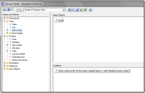
I built a first query that list stores :
The query became something like :
SELECT
 
Agg_yr_qt_mt_mn_wk_rg_cy_sn_sr_qt_ma.Store_name
FROM
  Agg_yr_qt_mt_mn_wk_rg_cy_sn_sr_qt_ma
Then, I based a query on it:
image
the query became :
SELECT
 
Article_lookup.Family_name
FROM
  Article_lookup,
  Outlet_Lookup,
  Shop_facts
WHERE
  ( Outlet_Lookup.Shop_id=Shop_facts.Shop_id  )
  AND  ( Article_lookup.Article_id=Shop_facts.Article_id  )
  AND  (
      @dpvalues('
Outlet_Lookup.Shop_name',9,1)@dpend
  )
at the next iteration, it became:
@dpvalues('
Outlet_Lookup.Shop_name',9,7)@dpend
and when I tried filtering for a number, it became:
@dpvalues('
sum(Agg_yr_qt_rn_st_ln_ca_sr.Sales_revenue)',536870916,12)@dpend

This tells me, it’s not a user-function. It’s an internal function. The user is expected to use a subquery instead.
Or, as Andreas stated on the forums :  query on query, which allows you to filter based on a different datasource.

Binabik


woensdag, november 16, 2011

An Exponential Trendline in Business Objects

This is going to be the third type of Trendline and I just noticed, Excel has six of them. I’m not sure how many really are used, or if there is a specific need for any in particular. So, for now, I’m gonna keep this at three, unless there is a demand for the other three. (Polynomial, Power and Moving Average).

I am going to add those three eventually, just for fun, but I’m going to keep them for a cold winter evening. Or when the question arises.

So, here’s the Exponential Trendline.

The magic number for the Exponential trendline is e. I’ve been reading about the constant e on Wikipedia and it’s a great story. You should read it too. One of the things I noticed is the amount of history that lies at the base of these trendlines. Amazing.

First, the formula:

Equation

Where c and b are constants. Each time when they say that (and here is where I find that info) I’m a bit pissed off. Especially, because they’re not constants at all. They’re calculated values. All of them.

c, as usual, is the intercept point but this time, it uses the Natural Logarithm of Y and the value (non Logarithm) of X. In fact, the calculation uses the EXP function, which is the inverse of a Natural Logarithm.

So, if i = ln(x), then exp(i) = x.

b is the coëfficient which we calculated in both other trendlines before, but this time, it uses the ln of  y.

(ah, on a sidenote, I wrote 2011 in my report, but on the test-databases that come with Business Objects, the numbers are identical for 2003 or 2006 –amazing huh Glimlach )

So, I take the ln on Sales Revenue and I call it LnY

The formulas are:

image

=ln(<Sales revenue> in body) in report (which is called LnY)

=Average(<LnY> in body) in Report (which I call AverageLnY)

Like in the linear trendline, we calculate X-AverageX where X is a Runningcount of the Month.

=((RunningCount(<Month>) In <Month>) - <AverageX>) In <Month>

=(<LnY> - <AverageLnY>) In <Month> becomes the variable LnY-AverageLnY

and we multiply those two :

=<LnY-AverageLnY>*<X - average X>

After which we add them up. As before, we now have the top of our division:

=Sum((<LnY-AverageLnY> * <X - average X>) In  Body) In Report

For the bottom part of our division, we need the Square of X-AverageX added up.

=Power(<X - average X>, 2) In <Month>

image

Now we divide those numbers

image

There, that’s our b-variable which we can use to calculate our c variable.

=<LnY>-(<LnCoeff>*<xvalue>)

image

There we go, we have both variables to put into our formula.

e = 2.71828, I found that on Wikipedia.

Now, one more thing needs to be done, and it’s probably why this is called the exponential trendline, we need to take the EXP of our intercept point (our c-variable)

=Exp(<InterceptLn>) In Report

image

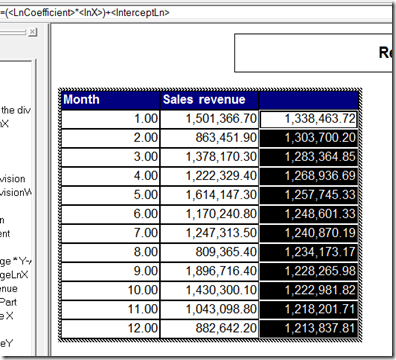
=<ExpIntercept>*(Power(2.71828 ,(<LnCoeff>*<xvalue>)))

this is the formulat shown at the top, turned Business Objects. We add that one and convert it to a table. That gives us the following chart:

image

And excel does this :

image

Again, a perfect match.

There. That gives you Linear, Logarithmic and Exponential trendlines to add to your charts.

Enjoy

Binabik

zondag, november 13, 2011

Logarithmic Trendline in Business Objects

Right, looks like I overestimated this one. After doing the previous one, Logarithmic just sounded a bit more scary. It really isn’t. In fact, it was the Microsoft site that got me a bit going. They mentioned something called “Linear Regression”. I looked up the math and it looked impressive. I had no idea, that was what I had already done in the previous article.

That has been my experience so far. A series of terms is unknown to me. This makes it fun to figure out how this stuff works because I really have to figure it out for myself.

Like the function in excel to calculate the Intercept point. On one site, I found this construction :

=index(linest(A1:A20;B1;B20);1)

Then, I found that the intercept function does exactly that. =intercept(A1:A20;B1:B20)

Ah well. it’s an amazing journey – and I’m enjoying every stop along the way.But without further ado, here’s the Logarithmic Trendline.

First off, the math is exactly the same as we had in the Linear trendline except that we don’t use x but ln(x). which is the natural logarithm of x.

for this, I use the function =Ln(runningcount(<Month>)) in <Month>

image

As with last time, I try to avoid using the month in a calculation, although it would work just the same.

Next up, we calculate the average of that column. In fact, that’s the only difference with the linear trendline.

image

=Average(LnX in Body) in Report is the function I use for that one.

image

Like with the linear trendline, we then need to make the difference between X and average X (this time with the logarithms of course) and Y- averageY.

=LnX – AverageLnX in Month

=Y – AverageY in Month

Next, we multiply those two with eachother and add them up.

image

=LnX-AverageLnX * Y-AverageY

=Sum(LnX-AverageLnX*Y-AverageY in body) in report

That last one is going to be the first part of our division.

image

Like last time, we now need to Square X-AverageX, but this time, it has to be the Ln version. So, the formula would be:

=sum(ln(x)-AverageLnX * ln(x)-AverageLnX  in body)in report

That’s going to be the second part of our division.

Next, we divide those two.

image

And we have our Direction Coëfficient.

Next up, we need the interception.

image

For this one, we need to subtract from AverageY

=<AverageY> – (<AverageLnX>*<LnCoëfficiënt>)

This formula, again, is the same as Linear trendline, but we use the one where we calculate the logarithm of X.

the next formula is : (Coefficient*LnX)+ InterceptLn

image

And then, we convert this baby to a chart.

image

And, it has the typical Logarithm curvature Glimlach

Here is the version Excel comes up with – and again, they are identical.

image

There. A logarithmic trendline is perfectly possible in Business Objects. One less reason to convert your Business Objects Report into an Excel sheet.

Next up : Exponential Trendline

Have a nice day !!

Binabik

donderdag, november 10, 2011

Trendlines in Business Objects

This is what we would want.A trendline in Business Objects.

image


It is not possible to let Business Objects insert a trendline in a chart automatically. It’s a feature that is simply missing. This is what I have been living with until now, it simply isn’t possible, end of story. And that makes me rebel. I want to make it possible.

Two problems : I’m not a real good mathematician. The math to achieve trendlines isn’t easy math either.

But, good news, I figured it out – and it works. Over the next few articles, I will hand you the math to add trendlines to your charts.

Our first type of trendline : A LINEAR TRENDLINE

The functions Excel uses to calculate that trendline looks like this :

and this

That’s the sort of math that makes my head spin – but after 5 minutes, I figured out how it works and then it’s easy. In case you don’t know, the x and y with a dash over their heads are averages.

The first function gets you the “direction-coëfficiënt”, the second gives you the interception point. Both are needed to calculate the trend.

Step1:

Calculate the average on both X and Y.
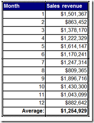
image

In this case, I used the formula : Average(<Sales revenue) in Report. If you don’t know what the “in Report” stands for, you should have a look at the articles about contexts. It’s not an easy subject.

With that, we have the average of Y and we also need the average of X. This might be a bit strange. Basically, you just need to find the middle of the X-axis of your chart.

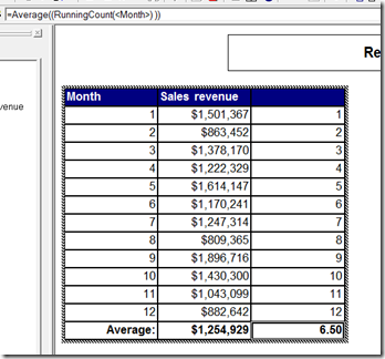
So, we need to count how many items there are and find the middle of that. In fact, for our 12 months the middle is not 6 but 6,5 because it’s an even number of lines. So, what I end up doing is using a runningcount function :”=RunningCount(<Month)” Which I then take an average on.
image

the function at the end is : =Average((RunningCount(<Month>) )) In Report. which I define as variable <AverageX>

This means, that at this point, we have the two numbers with the dashes over their heads. Next, we need to subtract the X and Y values from it.

For X, this is : =((RunningCount(<Month>) In <Month>) - <AverageX>) In <Month> which I define as a variable X – AverageX

image

Next, we need Y – AverageY

=(<Sales revenue> - <AverageY>) In <Month> which I define as Y – AverageY

image

Next, we need to multiply those : =<X - average X>*<Y - AverageY> and add them up.

image

This gives us the first part of our division, specified at the beginning of this document.

For our second part, we need to Square x-divisionX and add them up.

that’s :=Sum(Power(<X - average X> , 2) In  Body) In Report

image

Last but not least, we need to divide them to get the direction Coëfficient.
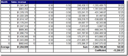
image

Now that we calculated b, we can proceed to calculate

This translates to :

=<AverageY> - (<AverageX>*<coefficient>)

and that’s our “Intercept” which amounts to the Intercept function in Excel.
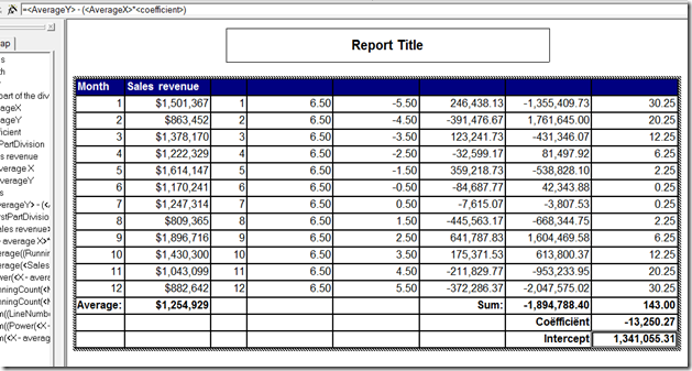
image

Now we can calculate the values for our Trendline. The function in this case (for a linear Trendline is:

y = mx + b

m = direction coëfficient

b = intercept

image

the x-Value is our runningCount on the month (rememberGlimlach)

So, now we transform this to a chart :

image

I had a great time trying to figure this one out, so I hope it’s useful to anyone. Next up Logarithmic trendlines. It won’t be easy, I can promise you that Glimlach


ah.. last but not least, this is what that trendline looks like in Excel Glimlach

image

Isn’t that – entirely – identical Glimlach Lovely.

Cheers

Binabik