Logarithmic Trendline in Business Objects

Right, looks like I overestimated this one. After doing the previous one, Logarithmic just sounded a bit more scary. It really isn’t. In fact, it was the Microsoft site that got me a bit going. They mentioned something called “Linear Regression”. I looked up the math and it looked impressive. I had no idea, that was what I had already done in the previous article.

That has been my experience so far. A series of terms is unknown to me. This makes it fun to figure out how this stuff works because I really have to figure it out for myself.

Like the function in excel to calculate the Intercept point. On one site, I found this construction :

=index(linest(A1:A20;B1;B20);1)

Then, I found that the intercept function does exactly that. =intercept(A1:A20;B1:B20)

Ah well. it’s an amazing journey – and I’m enjoying every stop along the way.But without further ado, here’s the Logarithmic Trendline.

First off, the math is exactly the same as we had in the Linear trendline except that we don’t use x but ln(x). which is the natural logarithm of x.

for this, I use the function =Ln(runningcount(<Month>)) in <Month>

As with last time, I try to avoid using the month in a calculation, although it would work just the same.

Next up, we calculate the average of that column. In fact, that’s the only difference with the linear trendline.

=Average(LnX in Body) in Report is the function I use for that one.

Like with the linear trendline, we then need to make the difference between X and average X (this time with the logarithms of course) and Y- averageY.

=LnX – AverageLnX in Month

=Y – AverageY in Month

Next, we multiply those two with eachother and add them up.

=LnX-AverageLnX * Y-AverageY

=Sum(LnX-AverageLnX*Y-AverageY in body) in report

That last one is going to be the first part of our division.

Like last time, we now need to Square X-AverageX, but this time, it has to be the Ln version. So, the formula would be:

=sum(ln(x)-AverageLnX * ln(x)-AverageLnX  in body)in report

That’s going to be the second part of our division.

Next, we divide those two.

And we have our Direction Coëfficient.

Next up, we need the interception.

For this one, we need to subtract from AverageY

=<AverageY> – (<AverageLnX>*<LnCoëfficiënt>)

This formula, again, is the same as Linear trendline, but we use the one where we calculate the logarithm of X.

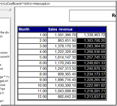
the next formula is : (Coefficient*LnX)+ InterceptLn

And then, we convert this baby to a chart.

And, it has the typical Logarithm curvature

Here is the version Excel comes up with – and again, they are identical.

There. A logarithmic trendline is perfectly possible in Business Objects. One less reason to convert your Business Objects Report into an Excel sheet.

Next up : Exponential Trendline

Have a nice day !!

Binabik